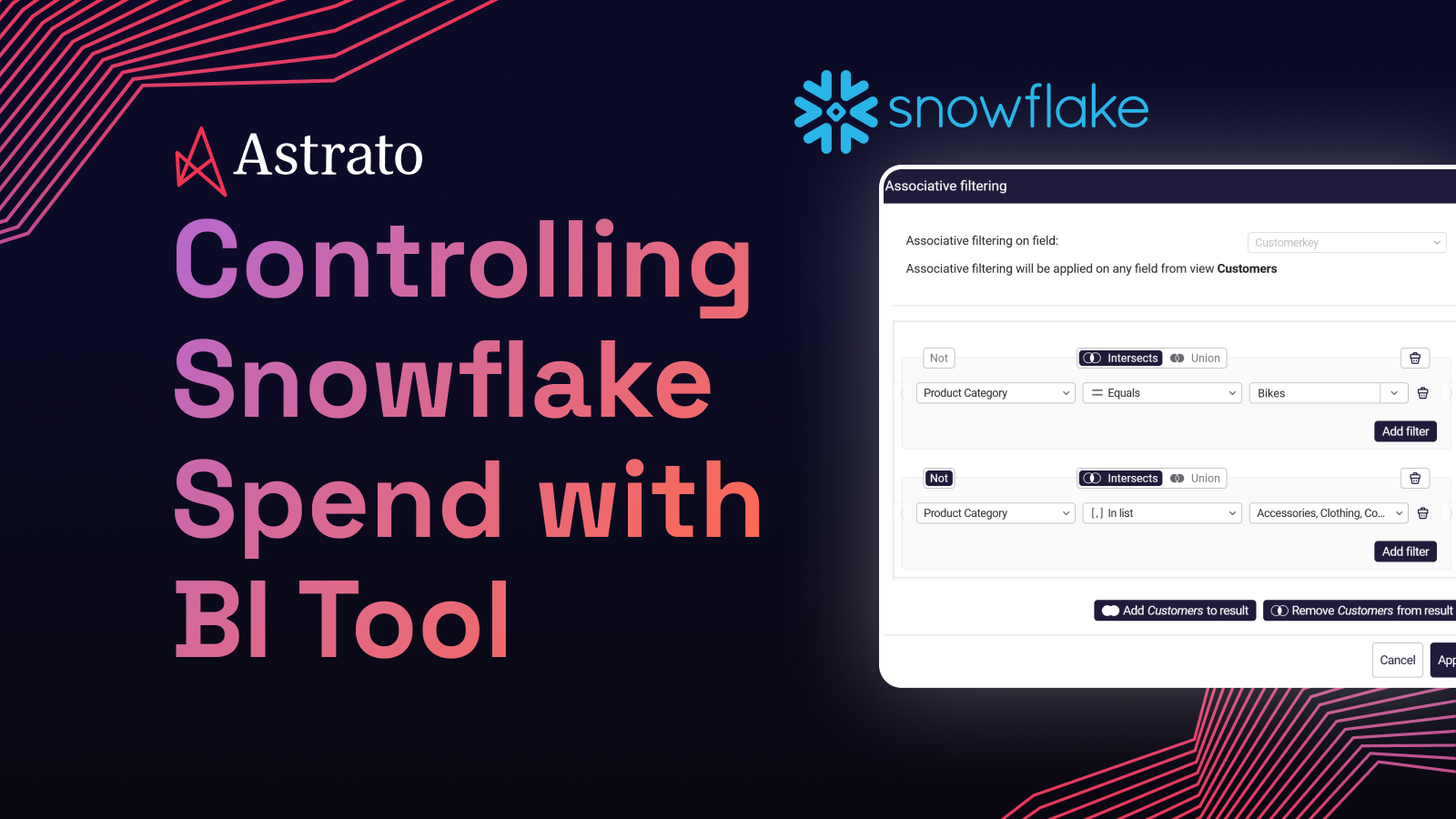
Controlling Snowflake Spend with Your BI Tool: Four-Lever Audit

The bill arrives, and finance has questions

You picked Snowflake because it scales with usage. It does. Now the bill scales with usage too, finance has noticed, and you're the one being asked what's driving it.

Most of the cost advice you'll find online splits in two directions. One half is Snowflake-side — warehouse sizing, auto-suspend timing, materialized views, resource monitors. Useful, but it treats your BI tool as a black box that “issues queries.” The other half is BI-vendor marketing — every platform claims to be the cheapest, none can prove it, and the strongest claims (Tableau extracts, Power BI Import, ThoughtSpot Falcon) are technically real but only on a narrow workload type.

Neither half answers the question you actually have: 

How does your BI tool change the shape of your Snowflake bill, and which architectural decisions are pushing it up?

This piece answers that. Snowflake spend on BI workloads moves on four levers — query frequency, query efficiency, cache utilization, and warehouse uptime. No tool wins on all four. The honest comparison isn't “which BI platform is cheapest” but “which platform's architecture aligns with the lever you most need to pull, and what trade-off you accept in exchange.”

By the end you'll have a four-lever framework you can apply to any vendor demo, an audit checklist you can run against your existing deployment in 30 minutes, and a rubric for matching architecture to workload — not a sales pitch dressed as a comparison.

TL;DR

Snowflake bills you for warehouse uptime, not query count, and gives you a free 24-hour result cache if your queries don't fragment it. Your BI tool affects four levers: how often it queries Snowflake, how efficiently each query runs, how well it aligns with the result cache, and how its query pattern shapes warehouse uptime. Live-query architectures push lever 1 up and unlock freshness; extract architectures push lever 1 down and trade staleness for raw compute savings. Pick the architecture that matches your workload's freshness needs and concurrency profile — not the one with the loudest cost claim.

How Snowflake actually bills BI workloads

Before you can map a BI tool to your bill, you need to know exactly how Snowflake is charging you. Three mechanics matter.

Per-second compute

Snowflake bills virtual warehouses by the second, with a 60-second minimum on every resume. A warehouse processing one query and a warehouse processing two hundred cost the same per second — until they hit capacity. So query count is almost a red herring. What you're really paying for is how long a warehouse stays awake.

Auto-suspend and the 60-second minimum

Auto-suspend lets a warehouse spin down when idle. The default is 600 seconds (ten minutes); the minimum is 60 seconds. Most teams accept the default and stop thinking about it. That's a mistake. If your BI tool issues a burst of queries every twelve minutes — say, a refresh job, a few exec dashboards, an embedded customer query — your warehouse never gets to suspend. It bills for ten idle minutes between every burst.

The result cache

Snowflake holds query results in a 24-hour cache, account-wide. If the same query (byte-identical SQL, same role, same data) is issued within that window and the underlying data hasn't changed, the result returns from cache without a warehouse spin-up. That's free compute. The catch is that the cache is exact-match: any parameter variation, timestamp injection, or role difference busts it.

Multi-cluster scaling

When concurrency exceeds what one warehouse can serve, Snowflake spawns a sibling cluster at the same per-second rate. This is invisible by design and often only shows up when the bill arrives. For multi-tenant analytics, it's the silent cost driver — a hundred customers hitting the same dashboard at 9 a.m. doesn't hit one warehouse harder, it spins up additional ones.

That's the billing surface your BI tool's behavior interacts with. Now the levers.

The four cost levers a BI tool can affect

Lever 1 — Query frequency

How often does your BI tool actually issue a query to Snowflake?

This is the lever where architecture diverges most starkly. A live-query tool like Astrato issues a query per chart per dashboard load. Open a dashboard with twelve charts, and Snowflake sees twelve queries (minus whatever the result cache catches). An extract-based tool like Tableau Hyper or Power BI Import issues a refresh on a schedule — once a day, once an hour — and serves every subsequent dashboard load from its own engine, not from Snowflake.

The arithmetic is straightforward. If your dashboard gets 1,000 loads a day and you're on a live-query tool, that's potentially 12,000 queries to Snowflake (less cache hits). If you're on Tableau with a daily extract, that's one refresh job — say, a heavier query that pulls the underlying data into Hyper — and 999 dashboard loads served entirely from Tableau's own compute.

For slow-changing data, extracts win this lever cleanly. For data that changes hourly or faster, the math inverts: extract-refresh frequency itself becomes the cost driver, and the live-query tool actually issues fewer queries because Snowflake's result cache catches the repeats. Astrato's session caching adds another layer here — identical queries within a user session don't re-hit the warehouse.

The honest characterization: extract architectures push lever 1 down at the cost of staleness; live-query architectures push it up in exchange for freshness and writeback. Neither is universally cheaper.

Lever 2 — Query efficiency (pushdown)

When a query does run, is it well-shaped SQL Snowflake can optimize, or naïve SQL that scans more than it needs to?

This is where architecture decisions show up as bytes scanned. A BI tool with strong pushdown sends Snowflake a tight query: filters in the WHERE clause, aggregations in the GROUP BY, joins where the join keys are clustered. A weak BI tool sends SELECT * FROM big_table and applies the filter in its own layer after pulling the rows back. Snowflake bills for the scan either way.

Looker is the strongest example of pushdown done well. LookML compiles to SQL that Snowflake's optimizer handles cleanly, and Looker's aggregate awareness layer can route a query to a pre-aggregated table when one exists. Astrato pushes filters, joins, and aggregations into SQL by default, and its semantic layer compiles to optimizer-friendly queries. Sigma's live-query mode does similar work on Snowflake. Tableau's Live Connection (DirectQuery to Snowflake) is more variable — pushdown depends on the workbook author, and naïvely-built workbooks frequently over-fetch.

The clearest test: pull a representative query from SNOWFLAKE.ACCOUNT_USAGE.QUERY_HISTORY, look at the BYTES_SCANNED field, and compare against the row count actually rendered in the dashboard. If you scanned 80 GB to render 200 rows, your BI tool isn't pushing filters down — it's pulling the data and filtering client-side. That's a lever 2 problem and it shows up directly on your bill.

Lever 3 — Cache utilization

Does your BI tool align with Snowflake's result cache, or fragment it?

The result cache is one of the most under-discussed cost levers in BI deployments. It's automatic, free, and instant — a 24-hour cache hit returns without spinning up a warehouse at all. But it's exact-match, which means how your BI tool constructs a query matters as much as what the query asks.

Two patterns fragment the cache. First, timestamp injection: BI tools that append ?_t=1730483920 style cache-busters to queries (often as a feature, “always fresh!”) never get a result cache hit. Second, parameter variation: tools that build SQL by string-concatenating filter values (WHERE region = 'EMEA') instead of binding them (WHERE region = ?) generate a unique query string for every filter combination, fragmenting the cache by user behavior.

Tools that align with the cache parameterize cleanly, avoid timestamp injection, and don't add proprietary cache layers that compete with Snowflake's. Astrato is strong here — it uses Snowflake's result cache by default and adds session-level caching on top, but it doesn't run its own cache layer that you'd be paying for separately. Looker is similarly clean. Tools with proprietary in-memory engines (ThoughtSpot Falcon, Power BI's tabular model) don't fragment Snowflake's cache so much as bypass it — different architecture, different trade-off.

For embedded multi-tenant deployments, this lever matters disproportionately. Hundreds of tenants hitting the same dashboard with the same filters can either share cache hits efficiently or each generate unique queries. The difference shows up as a warehouse uptime difference, which leads to lever 4.

Lever 4 — Warehouse uptime

Does your BI tool's query pattern keep warehouses busy, or let them auto-suspend?

This lever is the one BI buyers most often miss because it isn't visible in any single dashboard or query. It emerges from the pattern of queries across users and time.

A BI tool can scatter queries — small, frequent, irregular hits that keep a warehouse awake without keeping it usefully busy. Or it can cluster queries — concentrated bursts that justify a warehouse running, then long enough silence for it to suspend. Extract-based tools tend to cluster (refresh windows are heavy and concentrated). Live-query tools tend to scatter (queries follow user behavior, which is irregular).

The cost decision sits with you, not the tool: how you size warehouses and tune auto-suspend determines whether a scatter pattern is expensive or cheap. A 60-second auto-suspend on a small warehouse handles a scatter pattern efficiently. A 600-second default on an X-Large is the worst combination — you're paying for a big warehouse to sit idle between bursts.

For multi-tenant deployments, the question becomes whether to pool tenants on a shared warehouse (better cache utilization, occasional concurrency contention, multi-cluster spillover) or isolate them on dedicated warehouses (predictable per-tenant cost, more idle time, no cache sharing). The right answer depends on tenant size distribution. A pooled warehouse with multi-cluster scaling is usually the cost-efficient default; isolation only pays when you have a few large tenants whose load justifies their own resource.

This is the lever where your BI tool's behavior interacts most heavily with Snowflake-side discipline. Astrato doesn't choose your warehouse size or auto-suspend timing — those are your decisions. What it does affect is the query shape that hits those warehouses.

The live-query vs. extract trade-off, named honestly

The four levers all loop back to one architectural decision: live-query or extract.

Extract architectures (Tableau Hyper as default, Power BI Import as default, ThoughtSpot Falcon) genuinely cost less in raw Snowflake compute on slow-changing data with low-to-moderate concurrency. The math is honest: one daily refresh query is cheaper than a thousand interactive queries per day, even after cache hits. If your dashboards display data that changes weekly and your users tolerate 24-hour staleness, an extract-based tool will produce a smaller Snowflake bill.

It will not produce a smaller total bill, necessarily — extract tools have their own compute layer to license and run, whether that's Tableau Server capacity, Power BI Premium SKUs, or ThoughtSpot Falcon nodes. But the line item that says “Snowflake” will be smaller.

Live-query architectures cost more on lever 1 in exchange for everything else: data freshness, writeback, embedded customer-facing analytics, AI-powered exploration that needs current context, and operational workflows where a 24-hour-old dashboard is worse than no dashboard at all. They also benefit more from Snowflake's result cache, since repeat queries within 24 hours return free.

The trade-off is the article's most important sentence: extract architectures lower your Snowflake bill in exchange for staleness; live-query architectures raise per-session compute in exchange for freshness, action, and a unified architecture. If you've read our piece on real-time analytics on Snowflake, you've already seen this fork — same architectural decision, opposite reader question. There, the answer is “live-query, almost always.” Here, the answer depends on what your data does.

The savings Gray Decision Intelligence reports come from a combination — replacing Qlik's compute layer with warehouse-native execution, plus a different pricing model. The architectural piece is the durable one: when the BI tool stops maintaining its own engine, the line items it generated stop appearing on the bill.

The Kalibri case is the clearest illustration of when live-query economics win: heavy multi-tenant embedded analytics on a single Snowflake instance with datasets exceeding 100 billion rows, where any extract architecture would mean either stale data per tenant or refresh-job overhead multiplied by tenant count.

The semantic layer's role in cost control

A semantic layer is a cost lever even when nobody on your team frames it that way.

When a metric is defined in dbt, in a Snowflake view, or in your BI tool's modeling layer — and every dashboard pulls that definition rather than re-deriving “active customer” five different ways — your tool stops issuing five different SQL patterns to Snowflake. Cache hits go up. Pushdown gets cleaner. Materialized view alignment becomes possible because the view can be built against a known query pattern.

The flip side: when business logic lives in dashboards (Tableau calculated fields, Power BI DAX measures that don't compile cleanly to SQL), every dashboard generates its own query shape. Lever 2 suffers. Lever 3 suffers. The bill grows.

Astrato's semantic layer compiles to SQL Snowflake can optimize and works alongside dbt models rather than competing with them. Looker's LookML is the same idea, executed differently. Sigma supports semantic patterns through its dataset layer. Tableau and Power BI both have semantic modeling, but their modeling layers were designed around extract architectures, which means the cost benefits route through their own engines, not Snowflake's.

The deeper architectural point — why the semantic layer matters for building data products on Snowflake, not just for cost — is in our reference architecture piece. For this article, the takeaway is narrower: the semantic layer is a cost lever, and warehouse-native semantic layers stack with Snowflake's optimizer in a way that BI-tool-internal semantic layers don't.

The vendors compared, lever by lever

The four-lever rubric, applied across the seven embedded BI vendors most commonly evaluated against Snowflake. Read down a column for a vendor's profile; read across a row to see which architectures handle a single lever well.

Astrato

Live-query, no extracts, semantic-layer pushdown to SQL, no proprietary cache layer. Strong on lever 2 (efficiency) and lever 3 (cache utilization). By-design higher than extract tools on lever 1 (frequency); Snowflake's result cache and Astrato's session caching mitigate but don't eliminate this. Lever 4 (uptime) is a Snowflake-side decision Astrato doesn't control. Best fit for live data, customer-facing analytics, writeback workflows, and high-concurrency embedded use cases. Not the lowest-cost option for static historical dashboards over slow-changing data.

Sigma

Live-query primarily, with materialized data sets as an option for heavy workloads. Similar lever profile to Astrato — strong on pushdown and cache alignment, by-design higher on query frequency. Sigma's spreadsheet-style interface drives heavy ad-hoc query volume, which makes lever 4 (uptime) tuning especially important on large deployments.

Tableau

Extract-first by default (Hyper engine), DirectQuery to Snowflake as a secondary mode. Extracts genuinely win lever 1 on slow-changing data — you'll see fewer Snowflake queries and a smaller warehouse bill. Loses on freshness, which the cost article should acknowledge as an honest trade-off. DirectQuery mode is more variable; pushdown quality depends on workbook construction, and inefficient workbooks over-fetch. Tableau Server or Cloud capacity costs separately from your Snowflake bill.

Power BI

Import mode is the default and shifts compute from Snowflake to Microsoft's tabular engine. Your Snowflake bill drops; your Power BI Premium or Fabric capacity bill takes the slack. DirectQuery against Snowflake is supported but more expensive per session — DAX-to-SQL translation is less optimized than purpose-built warehouse-native tools. Microsoft Fabric's Direct Lake mode reads from OneLake, not Snowflake, so it sits outside this comparison entirely. Best fit for shops already on Microsoft capacity where the math of “shift compute to Power BI” works out.

Looker

Live-query against Snowflake via LookML, which compiles to optimizer-friendly SQL. Strong on lever 2 (pushdown) — among the best in the comparison. Aggregate awareness routes queries to pre-aggregated tables when available, which is a real cost lever. Doesn't run a proprietary cache layer competing with Snowflake's. Lever 1 profile is similar to Astrato's, with stronger aggregate routing and weaker session caching.

ThoughtSpot

Proprietary Falcon engine ingests Snowflake data and serves queries from its own in-memory layer. Lever 1 on Snowflake drops sharply — Snowflake mostly sees ingest traffic, not query traffic. Total cost picture depends on Falcon node sizing, which is a separate spend line. Best fit when Falcon's price-per-node math beats your Snowflake-equivalent compute on the workloads you'd otherwise run live.

Metabase

Live-query primarily, with a result-caching layer on top that can replace some Snowflake queries entirely. Decent mid-market cost profile — not as aggressive on pushdown as Looker or Astrato, not as cache-fragmenting as poorly-tuned Tableau Live. Cache layer adds operational complexity but can pay off on read-heavy workloads with stable filter combinations.

A cost audit checklist you can run in 30 minutes

If you have a Snowflake account and an existing BI deployment, you can find your actual cost driver in less time than a stand-up. Run these seven checks.

The checklist names no vendors. It's diagnostic, not prescriptive — the goal is to find your problem first, then decide what to do about it.

The decision: matching architecture to your workload

The right BI architecture for your Snowflake bill depends on three things: how often your data changes, how concurrent your users are, and how much staleness your workload tolerates.

Extract-first wins when data changes daily or less often, dashboard concurrency is low to moderate (a few hundred internal users, not thousands of customers), and 24-hour staleness is acceptable. Tableau Hyper, Power BI Import, and ThoughtSpot Falcon all fit this profile. Your Snowflake bill will be lower; your tool's compute bill will be separate.

Live-query wins when data changes frequently enough that extract refresh becomes the cost driver itself, the analytics are customer-facing (where staleness shows up as a product complaint, not just an internal annoyance), or the workload benefits from Snowflake's result cache through repeat queries. Astrato, Sigma, and Looker all fit this profile. Your Snowflake bill scales with usage; you don't pay for a separate compute layer.

Hybrid wins when your workload mixes — slow-changing historical dashboards alongside live operational ones. Most platforms with extract architectures also support live mode (Tableau, Power BI), and most live-query platforms support materialization patterns (Sigma, Astrato via Snowflake materialized views). The hybrid path is the most common reality for mature deployments and the hardest to evaluate cleanly during a vendor demo.

The cost case for warehouse-native architecture isn't that it's universally cheapest. It's that the line items align: you pay Snowflake for compute, and that's the entirety of the analytics compute bill. Adding extract engines, in-memory layers, or proprietary caches solves specific cost problems by introducing different ones.

If your evaluation is genuinely cost-led, this is the 9-criteria framework's criterion 9 deep-dived. Score this lever explicitly. Don't let it disappear into general “TCO” hand-waving.

FAQ

Does live-query architecture always cost more on Snowflake than extract-based BI?

No. For data that changes frequently (hourly or faster), extract refresh frequency becomes its own cost driver, and live-query architectures benefit more from Snowflake's automatic result cache. For slow-changing data with low concurrency, extracts genuinely produce a smaller Snowflake bill — but you pay separately for the extract engine's compute layer.

Which BI tool offers the best Snowflake cost governance?

There's no single answer because cost governance has multiple dimensions. Looker's aggregate awareness is among the strongest pushdown features in the category. Astrato's warehouse-native architecture eliminates the separate-compute-layer problem entirely. Tableau's extract model can dramatically reduce Snowflake queries on the right workload. The right tool depends on which lever your bill is most sensitive to.

How does Snowflake's result cache interact with BI tool caching?

Snowflake's result cache is exact-match and account-wide. BI tools that parameterize queries cleanly and avoid timestamp injection benefit automatically. Tools with proprietary cache layers (in-memory engines like ThoughtSpot Falcon or Power BI's tabular model) tend to bypass Snowflake's cache rather than complement it — different architecture, different cost trade-off.

Should you size one warehouse per BI tool, or one per tenant for embedded analytics?

Pooled warehouses with multi-cluster scaling are usually the cost-efficient default for multi-tenant deployments. They share cache hits across tenants and let Snowflake's auto-scaling handle concurrency spikes. Tenant isolation only pays when you have a few large tenants whose load justifies dedicated resources, or when contractual data isolation requirements rule pooling out.

Does writeback in a BI tool affect Snowflake costs?

Yes, but usually marginally. Writeback issues INSERT, UPDATE, or MERGE queries against Snowflake, which consume warehouse compute like any other query. The cost is small per write but worth modeling for high-volume workflows. Astrato's writeback runs under governed SQL through the same warehouse, so the cost is visible in the same QUERY_HISTORY you'd already be auditing.